Building a Color Summarizer using Clustering

Hello! In this blog post I wanted to share a cool application of unsupervised learning (using KMeans clustering but any clustering would work!). This is a project I did a while ago but here I present you a polished version.

This time I’ll be making a color clustering script. The idea is to understand each pixel’s colour as a 3 variable observation (Red,Green and Blue). By calculating proximity between colours, we could reduce the number of colors in a picture. This has some potential applications as image segmentation, simplifying shapes in the image and detecting potential different objects. Let’s jump into it:

Load the picture

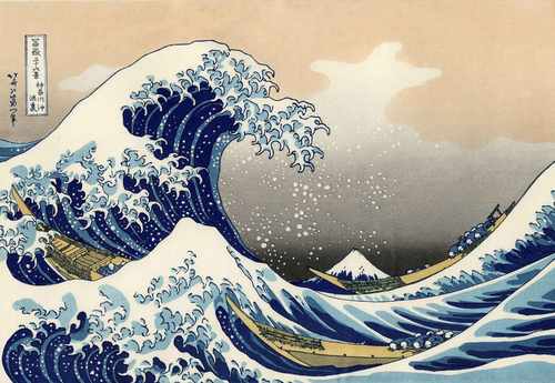
This cell is used to load the picture and resize it using Pillow. I’m using the Great Wave off Kanagawa, a really cool painting from the Edo period by Katsushika Hokusai as an example

from PIL import Image
import numpy as np

#Read Image
route="./wave.jpg"
img=Image.open(route,"r")

#Resize to be 500x500 maximum
if (img.size[0]>500) or  (img.size[1]>500):
  print("Picture too big, resizing")
  factor=500/max(img.size[0],img.size[1])
  new_size=tuple(i*factor for i in img.size)
  img.thumbnail(new_size,Image.ANTIALIAS)

#Save the shape for future use
original_shape=np.array(img).shape
print(original_shape)
img

Picture too big, resizing
(345, 500, 3)

Converting the image into a dataframe

There is no need to do this step but it gives a good idea on how to interpret the pixels as observations of three variables.

import pandas as pd
def img_to_df(img):
  R=np.array(img.getdata(band=0))
  G=np.array(img.getdata(band=1))
  B=np.array(img.getdata(band=2))

  df_img=pd.DataFrame({"R":R,"G":G,"B":B})
  return df_img

df_img=img_to_df(img)
df_img

	R	G	B
0	240	226	200
1	240	225	200
2	240	225	201
3	240	225	202
4	239	224	203
...	...	...	...
172495	131	168	180
172496	134	171	183
172497	131	168	180
172498	123	160	172
172499	128	165	177

172500 rows × 3 columns

Plotting the observations in the 3 Axes

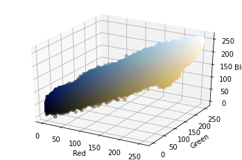
As you can see in the following 3D graph, we can plot each pixel represented by its own color in a 3D graph. Since this image uses quite distinct colours, we can see four regious, from the darkest colours around the (0,0,0) to the whitest at the (255,255,255). Keep in mind we are using the RGB model, so each colour is represented by adding Red, Green and Blue, each one ranging from 0 to 255.

import matplotlib.pyplot as plt

def plot_3d_pixels(df_img,colors):
  fig = plt.figure()
  ax = plt.axes(projection='3d')

  ax.scatter(df_img["R"],df_img["G"],df_img["B"], c=colors, marker='o')

  ax.set_xlabel('Red')
  ax.set_ylabel('Green')
  ax.set_zlabel('Blue')

  plt.show()

plot_3d_pixels(df_img,colors=[tuple(i/255) for i in df_img.values])

Fitting the clustering algorithm

Just as I said above, you can fit the clustering using pixels as observations and R,G,B as variables. the following cell simply does that, using the fit_clust function which takes the data, the clustering function and the arguments for that algorithm as a dictionary

from sklearn.cluster import KMeans,SpectralClustering

def fit_clust(X,clust_func,clust_args): #Fit the clust_func clustering algorithm
  
  clust=clust_func(**clust_args)
  clust.fit(X)
  return clust

clust_params={"n_clusters":3}
clust=fit_clust(df_img,KMeans,clust_params)

Swapping colours

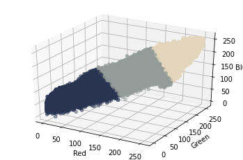
Once the cluster is set, we just have to change each pixel’s colour to their corresponding centroid colour (since we are using kmeans, the average of all colours in that cluster). In the following 3D graphs we can see how the colours were determined.

To be honest, other clustering algorithms might provide better results, since KMeans mainly provides spherical clusters. I haven’t tried normalization either since the 3 variables we are using (RGB) are on the same scale.

def swap_colors(clust,shape):
  labels=clust.labels_
  colors=clust.cluster_centers_
  colors=np.array([tuple(i) for i in colors])
  return colors[labels].reshape(shape)

def build_image_from_cluster(clust,shape):
  new_pixels=swap_colors(clust,shape)
  return Image.fromarray(new_pixels.astype('uint8'), 'RGB')


new_image = build_image_from_cluster(clust,original_shape)

plot_3d_pixels(df_img,colors=[tuple(i/255) for i in img_to_df(new_image).values])
plot_3d_pixels(df_img,colors=[tuple(i/255) for i in df_img.values])

Final Result

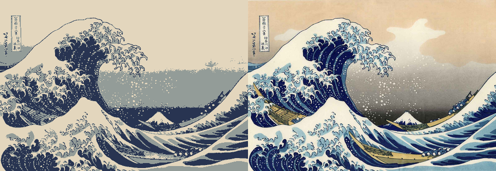
Here is the final result!

new_image.save("clustered_img.jpg")
new_image

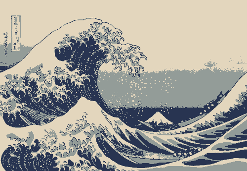
And here is the “summarized image” side to side with the original one. Looks like a newspaper adaptation.

paste_img = Image.new('RGB', (img.size[0]*2,img.size[1]))
paste_img.paste(new_image, (0,0))
paste_img.paste(img, (img.size[0],0))
paste_img

Using more clusters

As you may’ve imagined, the more clusters you use, the more vivid the image will be. This code below creates a gif showing how the image changes when increasing the number of clusters (colors) to sumarize the image with

from PIL import ImageFont
from PIL import ImageDraw 

#Adding text to the image
def label_image(img,text,pos):
  img = image
  draw = ImageDraw.Draw(img)
  font = ImageFont.load_default()
  draw.text(pos,text,(255,0,0),font=font)
  return img

import imageio
images = []

# Building the Gif
for nclust in range(1,15):
  print("Fitting with",nclust,"clusters")
  clust=fit_clust(df_img,KMeans,{"n_clusters":nclust})

  image=build_image_from_cluster(clust,original_shape)
  image=label_image(image,"Nclust="+str(nclust),(original_shape[1]-55,0))
  images.append(np.array(image))

#Repeating last frame to check the final result
for i in range(3):
  images.append(images[-1])
imageio.mimsave('movie.gif', images,duration=1.5)

Fitting with 1 clusters
Fitting with 2 clusters
Fitting with 3 clusters
Fitting with 4 clusters
Fitting with 5 clusters
Fitting with 6 clusters
Fitting with 7 clusters
Fitting with 8 clusters
Fitting with 9 clusters
Fitting with 10 clusters
Fitting with 11 clusters
Fitting with 12 clusters
Fitting with 13 clusters
Fitting with 14 clusters

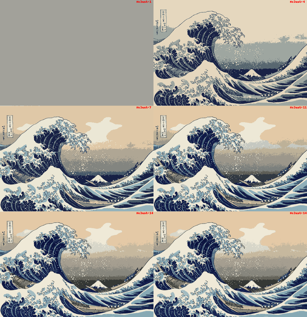
Here is another example with a couple of Macaws I created using the script.

If you want to try it, I Uploaded it to Google Collab. You just have to upload the picture and change the route at the beginning and it will be processed in Google’s Servers so you don’t need a powerful computer!

Hope you enjoyed the post! Feel free to ask me if you have any questions!