Do your samples follow the same distribution? Kolmogorov-Smirnov test from scratch!

When we run any kind of data-based study in order to model reality, we sometimes assume that our data is static. This is usually the case for research in which, once the dataset has been created, it’s never updated. However, in the real world/industry, data changes; consumer behaviours, climate patterns, you name it! It can also be used to be if your train-test data splits of a continuous variable are equally distributed.

In this blog post I’ll show you how to study this phenomena with one test that has stood the test of time: the Kolmogorov Smirnov test. You’ll learn an approximation to how the test was derived, assuming that you have a minimal knowledge of statistics (any basic subject that you have taken will do). Keep in mind that the mathematics/procedures might not be very pure/robust but I think it’s better to explain it this way

Empirical distribution function and Gilvenko-Cantelli

The Kolmogorov-Smirnov test relies on the Fundamental Theorem of Statistics (a.k.a Gilvenko-Cantelli theorem).

Do not get scared by mathematical notation. I will try to explain everything in plain english after bombarding you with maths.

Let $X_1,\ldots,X_n$ be our random sample of independent, identically distributed ($i.i.d$) samples. This is, we collect a group of individuals/observations that follow an “probabilistic behaviour” (that’s why they are observations of a random variable $X$) that regulated the value we observed, which we do not usually know. Most of the time we just say this is a normal distribution, but there are plenty of them.

We can compute the empirical distribution function:

\[\hat{F_n}(x) = \frac{1}{n} \sum_{i=1}^{n} I_{(-\infty, X_i]}(x)\]

This function is an aproximation to the cumulative distribution function, cdf, also named probability function $F$. What it represents is that, given any value $x$ the proportion of values $X_i$ in our sample that were smaller than $x$. This proportion stablishes an analogy to probability (the probability of any observed sample being smaller than $x$, $P(X<x)$ is similar to the proportion of items we saw smaller than X), so that

\[P(X \leq x) = F(x) \simeq \hat{F_n}(x)\]

Going back to Gilvenko-Cantelli. This theorem states that for every fixed $x$, $\hat{F}_n$ converges to the actual cumulative distribution function $F$. This is guaranteed through the law of the great numbers, but Gilvenko and Cantelli proved uniform convergence, stating that:

\[{\displaystyle \|F_{n}-F\|_{\infty }=\sup _{x\in \mathbb {R} }|\hat{F}_{n}(x)-F(x)|\longrightarrow 0} \text{ almost surely}.\]

In plain english, what does this (roughly) mean? As we gather more samples (we make $n$ larger), our empirical distribution function will start to look more like the one that ruled our sample, because the maximum ($sup$) difference between $F$ and $\hat{F}_{n}$ will shrunk towards 0. This does make sense, right? As we observe more randomly sampled individuals, we will have more information about the probabilistic behaviour that regulated our sample.

We can simulate an example here. Let’s use a good’ol normal distribution:

import numpy as np
import matplotlib.pyplot as plt
from scipy.stats import kstest
from scipy.stats import norm

np.random.seed(0)
def edf(sample: np.array):
  return np.arange(len(sample))/float(len(sample))

fig, axs = plt.subplots(3,1, figsize=(5,10))

diffs = {}
F_hat = {}
X = {}
ns = [2**i for i in range(2, 13, 1)]
for n in ns:
  sample = np.random.normal(size=n)
  X[n] = np.sort(sample)
  F_hat[n] = edf(X[n])
  diffs[n] = np.abs(F_hat[n] - norm.cdf(X[n]))


for n in ns[4:]:
  axs[0].plot(X[n], F_hat[n], label=f'n={n}')
  axs[1].plot(X[n], F_hat[n], label=f'n={n}')
  axs[2].plot(X[n], diffs[n], label=f'n={n}')

for ax in axs[0:2]:
  ax.plot(X[n], norm.cdf(X[n]), label='F', linestyle='dashed')

for ax in axs:
  ax.legend()

axs[1].set_xlim(-0.5, 0.5)
axs[1].set_ylim(0.4, 0.6)

axs[2].set_xlim(-2, 2)

axs[0].set_ylabel('F_n')
axs[1].set_ylabel('F_n zoomed')
axs[2].set_ylabel('|F-F_n|')

plt.show()

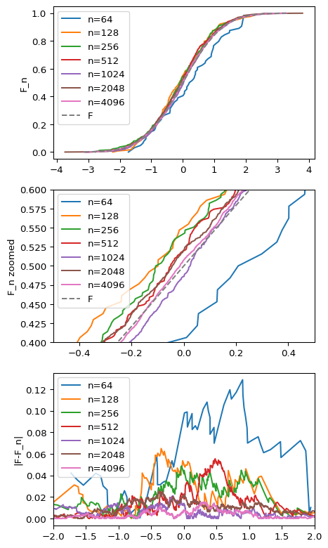
Here, we can see two interesting outcomes. First, $\hat{F}_n$ starts looking more and more like $F$ as $n$ grows (first and second plot). In fact, for the largest samples differences are barely noticeable due to scale. Secondly, as $n$ decreases, the maximum difference shrinks. So empirically the theorem holds!

Kolmogorov-Smirnov

The Kolmogorov-Smirnov test has two uses:

• Test if your sample $X_1,\ldots, X_n$ was drawn from a distribution (for instance, is my data $N(0,1)$ distributed?).
• Test if two samples $X_1, \ldots, X_n$ come fom the same distribution

I’ll focus on the two sample test as this is more interesting for real world ML applications. Let’s think about the following situations:

• You are trying to check if a new cheaper-to-produce product (this can be a machine learning algorithm!) you are giving to your costumers is behaving the same way as the one you were using before.

• You want to check if any of your predictors drifted (your model was trained on one input distribution but you are afraid that suddenly this distribution has changed because of external factors. Your model should be retrained in order to capture this change in concept).

Let’s place these problems in the framework we looked at in the beginning.

• Let $X_1, \ldots, X_n$ be old independent observations that used your own technique/product/model (i.e you collected before)
• Let $Y_1, \ldots, Y_n$ be new independent observations after applying your new technique/product/model (i.e. you collected them just now)

We want to check if these two samples were drawed from the same distribution.

Remember what Gilvenko-Cantelli studied?:

\[\sup _{x\in \mathbb {R} }|\hat{F}_{n}(x)-F(x)|\]

We can refactor this, where $F^x$ and $F^y$ would be the cdf of each sample to:

\[D^{xy+}_n = \sup _{x\in \mathbb {R} }|\hat{F}^x_{n}(x)-\hat{F}^y_{n}(x)|\]

Now, we can study $D_n^{xy+}$ which is basically the largest of the differences between the observed $\hat{F}$s.

Let’s use synthetic data again. We are going to generate three samples of 20 individuals, from three random variables $X$, $Y$ and $Y_d$, where $X$ and $Y$ follow the same distribution but $Y_d$ has a slight drift

n = 20
mu1 = 5
mu2 = 6
sigma1 = 2
sigma2 = 2.2

X = sorted(np.random.normal(size=n, loc=mu1, scale=sigma1))
Y = sorted(np.random.normal(size=n, loc=mu1, scale=sigma1))
Y_d = sorted(np.random.normal(size=n, loc=mu2, scale=sigma2))

F_x = edf(X)
F_y = edf(Y)
F_yd = edf(Y_d)

fig, axs = plt.subplots(2,1, figsize=(5,10))
axs[0].plot(X, F_x, label='X')
axs[0].plot(Y, F_y, label='Y same dist')
axs[0].plot(Y_d, F_yd, label='Y drifted')

axs[1].hist(X, alpha=0.5, label='X')
axs[1].hist(Y, alpha=0.5, label='Y same dist')
axs[1].hist(Y_d, alpha=0.5, label='Y drifted')


for ax in axs:
  ax.legend()
plt.show()

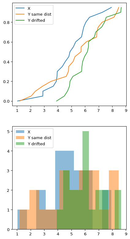
Even when we know that $X$ follows the same distribution than $Y$ but different than $Y_d$, it’s kind of hard to eyeball whether this is the case or not by looking at the plots although you can see that the green drifted distribution seems to behave different. The difference in $\mu$ and $\sigma$ is pretty large for that one. But if I didn’t tell you $X$ and $Y$ followed the same distribution, would you be able to give a robust assesment?

We can set a hypothesis and test it: $X$ and $Y$ come from the same distribution. When we say hypothesis, this is a claim that we assume to be true, and we see if it made sense to observe what we have observed if it was true through a hypothesis test.

If our data does not back up our claim, we will reject it. This will be reflected through a low p-value (I won’t go deep in the topic of mispractices in hypothesis testing, but let’s say that low p-value => our data does not back up our null hypothesis). So, with that in mind, one could think that if $X$ and $Y$ are very similar, $D^{xy+}_n$ (the maximum difference of their empirical distribution functions) has to be veeery little, close to 0 even. Wait, this is exactly what Gilvenko-Cantelli was talking about! So, we could test something similar to:

$H_0: D^{xy+}_n \text{ is very very small}$

And this is exactly the Kolmogorov-Smirnov test does: it studies the behaviour of the maximum of the differences in the empirical distribution function! The distribution of $D^{xy+}_n$ is derived from the brownian bridge (as usual, K-S test wikipedia page is a good first approach to the topic), but we won’t worry about this today. Luckily, we have the test implemented for us in python in the scipy.stats library.

X vs Y:

kstest(X,Y)

KstestResult(statistic=0.25, pvalue=0.571336004933722)

X vs Y drifted

kstest(X, Y_d)

KstestResult(statistic=0.4, pvalue=0.08105771161340149)

We can see that our null hypothesis is not rejected for the first test, but would be rejected at level $\alpha=0.1$ for the second test. If we repeat the experiment with a larger sample size

n = 500
X = np.random.normal(size=n, loc=mu1, scale=sigma1)
Y = np.random.normal(size=n, loc=mu1, scale=sigma1)
Y_d = np.random.normal(size=n, loc=mu2, scale=sigma2)

kstest(X,Y), kstest(X, Y_d)

(KstestResult(statistic=0.058, pvalue=0.3699050405997647),
 KstestResult(statistic=0.236, pvalue=1.2717086973677652e-12))

We can see that the test would be rejected for the drifted distribution $Y_d$, but not for the $X,Y$ pair.

Problems with the Kolmogorov Smirnov test

I just showed you that the test behaves well with a larger sample. But this can be problematic too! The main critics towards the Kolmogorov-Smirnov test come from the fact that it’s too sensitive to any kind of difference between the underlying distribution functions, only applicable in a single dimension and is biased depending on the sample sizes

It also may be problematic with members outside the exponential distributions family and with heavy tails since these tend to converge much slower or don’t even converge(as the differences all matter the same when computing the test statistic, I won’t be trying to prove this so take it with a grain of salt). There is no other better candidate to torture this test than the Cauchy distribution!

from scipy.stats import cauchy

p_c = []
p_n = []
B = 100
for n in ns:

  p_c_r = []
  p_n_r = []
  for rep in range(B):
    np.random.seed(rep)
    X_c = cauchy.rvs(size=n, loc=1, scale=2)
    Y_c = cauchy.rvs(size=n, loc=1, scale=2.5)

    X_n = np.random.normal(size=n, loc=1, scale=2)
    Y_n = np.random.normal(size=n, loc=1, scale=2.5)


    p_c_r.append(kstest(X_c,Y_c).pvalue)
    p_n_r.append(kstest(X_n,Y_n).pvalue)
  
  p_c.append(np.mean(p_c_r))
  p_n.append(np.mean(p_n_r))

plt.plot(ns, p_c, label='Cauchy')
plt.plot(ns, p_n, label='Normal')
plt.ylabel(f'average p value over {B} repetitions')
plt.axhline(0.05, linestyle='dotted', label="$ \\alpha = 0.05 $")
plt.legend()
plt.show()

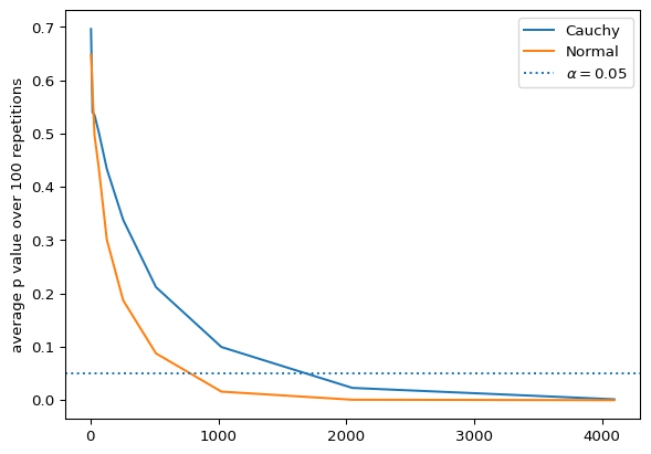
We can see how with a heavy tailed distribution like the Cauchy, the test takes longer to reach a confident rejection. As usual, don’t blindly trust the p-value!

ML-Ops use case:

Let’s look at a particular usecase to detect data-drift. We are building a classifier with $X_o$, a normal bivariate sample, which true label comes from a simple rule: 1 if the value is below the mean sample in both components, 0 otherwise. I won’t be doing train-test splits as we are doing a very basic example.

import matplotlib.pyplot as plt
import numpy as np
from sklearn.linear_model import LogisticRegression
n = 400

mu_o = 5

def get_data(mu): 
  return np.random.multivariate_normal(size=n*2, mean=[mu,mu], cov=np.eye(2))
def get_labels(X): 
  return (X[:,0]<X[:,0].mean()) + (X[:,1]<X[:,1].mean())

def plot_scatter(X, Y, **kwargs):
  levels = np.unique(Y)
  for level in levels:
    level_idx = Y==level
    plt.scatter(X[level_idx,0],X[level_idx,1], **kwargs, label=str(level))
    plt.legend()


X_o = get_data(mu_o)
Y_o = get_labels(X_o)


plot_scatter(X_o, Y_o, marker='$o$')

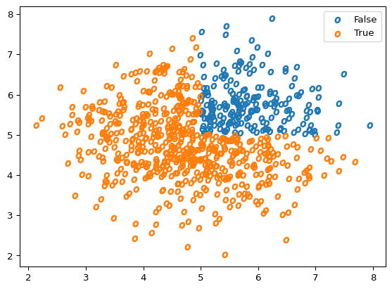
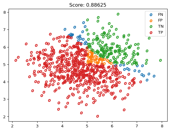
If we fit a Logistic Regression, we can see how well we did when predicting the labels.

def results_vector(y, yhat):

  tp = np.logical_and(yhat, y)
  tn = np.logical_and(~yhat, ~y)
  fp = np.logical_and(yhat, ~y)
  fn = np.logical_and(~yhat, y)

  labels = np.empty(dtype=object, shape=tp.shape)
  labels[tp] = 'TP'
  labels[tn] = 'TN'
  labels[fp] = 'FP'
  labels[fn] = 'FN'
  
  return labels

reg = LogisticRegression().fit(X_o, Y_o)
Y_hat_o = reg.predict(X_o)
plot_scatter(X_o, results_vector(Y_o, Y_hat_o), marker='$o$')
plt.title(f"Score: {reg.score(X_o, Y_o)}")
plt.show()

Now it comes the data drift. Suddenly, the data drifted (in a real life situation, you wouldn’t know this beforehand, this method would allow you to monitor those drifts in production) in one component, this is our observations will still follow the same rule to get their label but now their mean has changed, so the relation between X_d and Y_d is different

drift = 1

X_d = X_o.copy()
X_d[:, 0] +=drift
Y_d = get_labels(X_d)

plot_scatter(X_o, Y_o, marker='$o$')
plot_scatter(X_d, Y_d, marker='$d$')

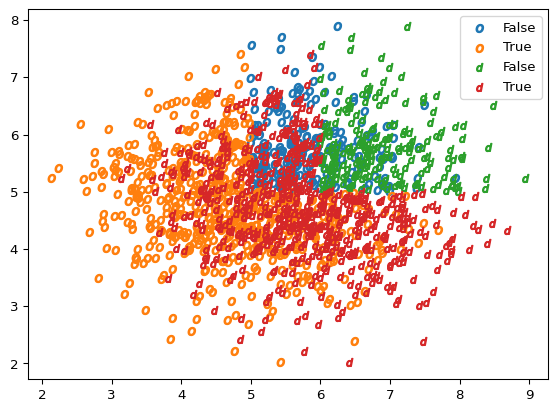
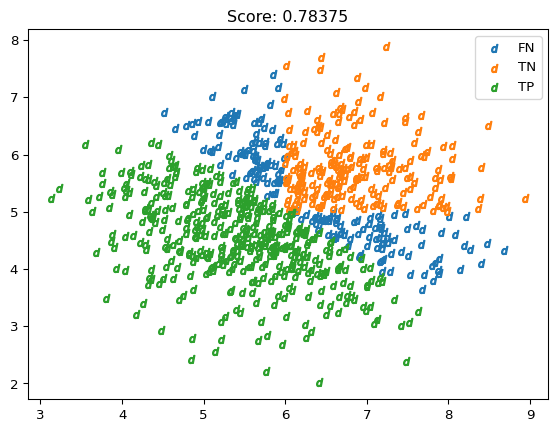
As we can see, the new data cloud (represented with $d$s) has drifted slightly towards the right side of the plot. If we predict on our new data, we can see the score has dropped and that we predict a lot of False negatives, with our score having decreased and the model producing no false positives

Y_hat_d = reg.predict(X_d)
plot_scatter(X_d, results_vector(Y_d, Y_hat_d), marker='$d$')
plt.title(f"Score: {reg.score(X_d, Y_d)}")
plt.show()

plot_scatter(X_o, results_vector(Y_o, Y_hat_o), marker='$o$')
plot_scatter(X_d, results_vector(Y_d, Y_hat_d), marker='$d$')

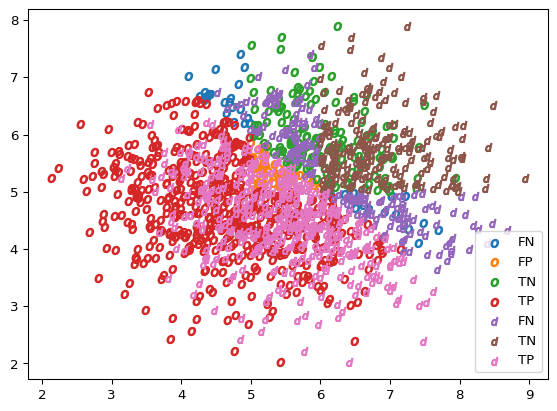
If we run the KS test on this drifted variable

kstest(X_d[:, 0], X_o[:, 0])

KstestResult(statistic=0.3775, pvalue=3.750151509284824e-51)

We can see that the test is able to detect the drift we inducted in the data since we have a small p-value.

Summary

With this blog post, we’ve:

• Seen how was the KS test constructed
• Seen python implementations
• KS test caveats
• A practical example on how to use this test

There are other alternatives that I’ll talk about in a different post, such as the Cucconi test and the Lepage Test. Hope you enjoyed the post!